Cyclic Schedules and the Max-Plus Eigenvalue
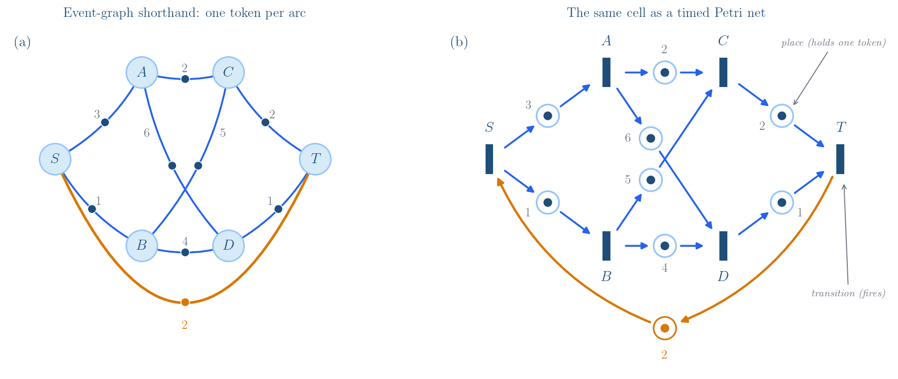
Picture a small assembly cell. Its product is a unit of two modules, joined at final assembly \(T\): a \(C\)-module and a \(D\)-module, each combining one \(A\)-side and one \(B\)-side component. A release at \(S\) starts the two fabrication stages: every firing of \(A\) makes a matched pair of \(A\)-side components — one bound for \(C\), one for \(D\) — and \(B\) does the same for the \(B\)-side. Each arc weight is an availability lag (transport, curing, inspection), and an assembly join fires once every component feeding it has arrived — incoming arcs mean “wait for all,” never “pick one.” One extra arc closes the loop: completing a unit at \(T\) frees an authorization card that travels back to \(S\) (lag 2), and the next kit of raw material is released only when a card arrives — the pull rule of a CONWIP/kanban cell. That back-edge turns the one-shot schedule into a cyclic event system, governed by the max-plus recurrence
\[x_j(k+1) = \max_i \bigl( x_i(k) + \widehat{P}_{ij} \bigr),\]
where \(x_j(k)\) is the time of the \(k\)-th firing of stage \(j\). After a transient, such a system is eventually periodic up to linear drift: the relative pattern of event times repeats while advancing at a fixed rate. That rate is an eigenvalue — the maximum cycle mean — and the cycle that attains it is the system’s bottleneck.
The graph itself belongs to a named family: it is a timed event graph, the choice-free subclass of Petri nets in which every place has exactly one producer and one consumer. Redrawn as a Petri net, the six stages become transitions (the things that fire), the nine streams — including the returning card — become places, the one-item-per-arc assumption becomes an initial marking of one token per place, and the weights become holding times. “Wait for all” stops being a convention declared from outside and becomes geometry: arcs converging on a transition can mean nothing else. Choice-freeness is exactly what makes the timing dynamics max-plus linear; the paper’s Petri-net appendix (Appendix D) develops the correspondence.
Tropical multiplication accumulates lag around the loop. The worst cycle sets the beat.
The explorer is a single self-contained HTML file. It runs entirely in your browser with no server, no network, and no dependencies — so the Download offline HTML link above gives you the same artifact to keep and open directly from disk.
What you can do
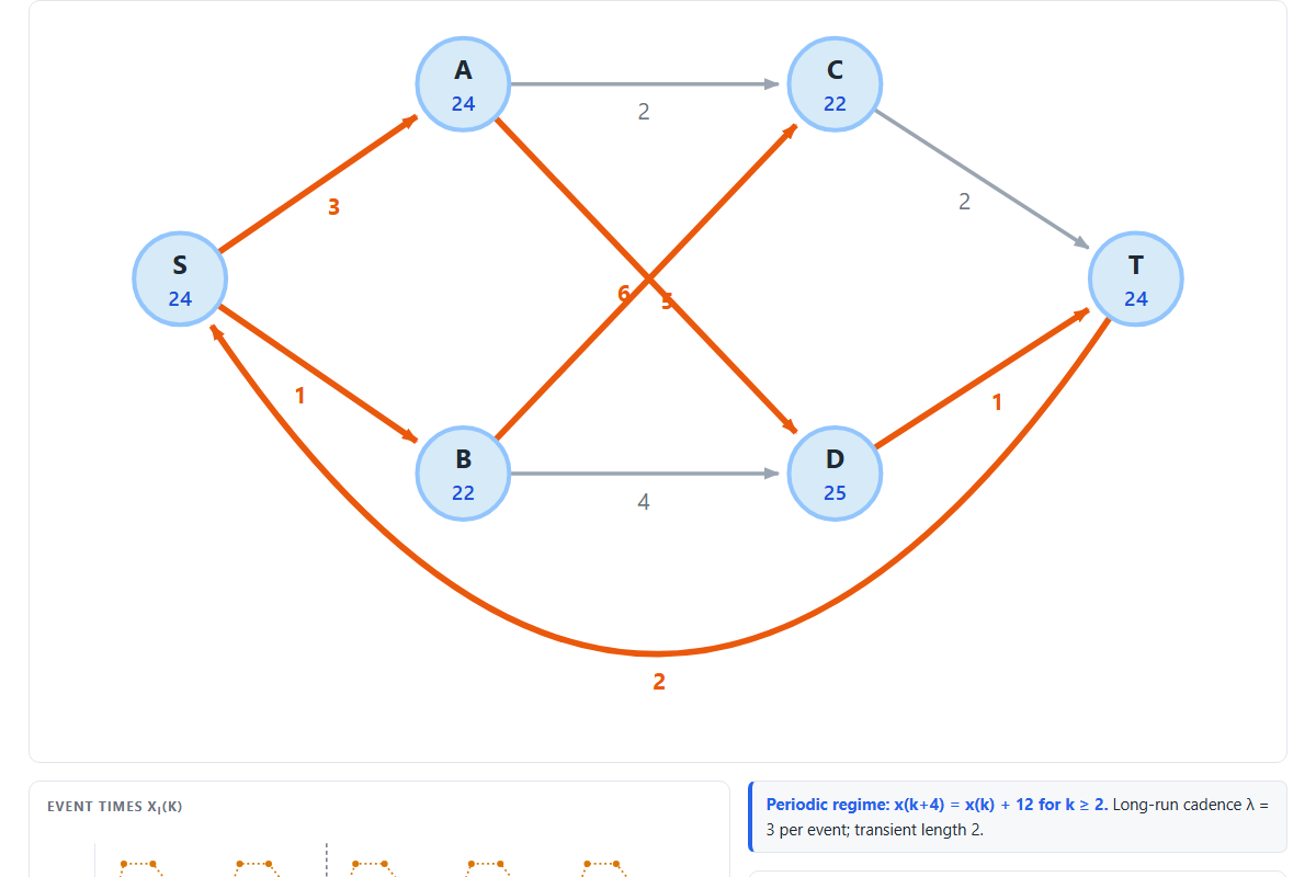
- Step the recurrence from a chosen initial vector and watch the transient lock onto the periodic regime \(x(k+4) = x(k) + 12\) — twelve time units every four events, a cadence of \(\lambda = 3\).
- Flip the chart to de-trended view \(x(k) - \lambda k\): the periodic regime becomes a flat repeating band, and the system’s drift disappears.
- Start from the eigenvector \(v = (0, 0, -2, 0, 3, 1)\) and see the special case: no transient, no wobble — \(x(k) = v + 3k\) exactly.
- Drag arc weights in the sensitivity view: watch the four cycle means, the eigenvalue, and the critical cycle respond. Speeding up an off-bottleneck arc changes nothing; slowing the transfer \(A \to D\) to 4 produces two co-critical cycles — the exact breakpoint in the piecewise-linear curve \(\lambda(w)\).
- Toggle the semantics view between the one-kit-at-a-time reading (one unit per 12 time units) and the pipelined first-order reading (one per \(12/4 = 3\)): same graph, same weights — the bottleneck cycle’s 12 time units of lag amortized over its four items of work in progress.
This artifact covers the cyclic half of the story; the one-shot half — shortest paths, Bellman–Ford, and critical paths on the same graph — lives in the shortest-paths explorer.
Supporting information
This page is supporting information for the tropical-algebra paper When Addition Becomes Optimization: Tropical Algebra, Paths, Schedules, and Semiring Computation (Sections 9–10: cyclic event systems and max-plus eigenvalues; the Petri-net appendix, Appendix D, places the event graph within the wider Petri-net family). It is designed to remain usable offline and is archived on Zenodo alongside the paper, where the five explorers ship together as a downloadable bundle.